Application Note AN622001

APPLICATION
The Solar Type 6220-1B Audio Isolation Transformer was especially designed for screen room use in making conducted audio frequency susceptibility tests as required by MIL-STD-461/462 and other EMI specifications.

The transformer may also be used as a pickup device to measure low frequency EMI currents at lower levels than conventional current probes.

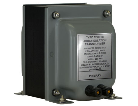
USE OF THE TYPE 6220-1B TRANSFORMER IN GENERAL
Since the transformer is connected in series with each ungrounded power input lead (sequentially) for performing the audio susceptibility tests, it can be used for two additional purposes while still in the circuit. First, the secondary winding can act as the series inductor suggested for transient injection tests to prevent the transient from being short-circuited by the impedance of the power line. In this application all other windings are left open (see Figure 1). Secondly, the transformer can be used for measuring EMI current as described herein (see Fig. 2).

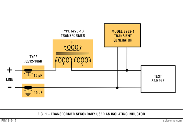
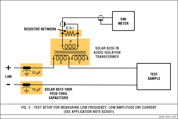
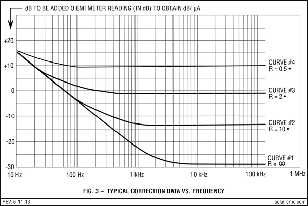
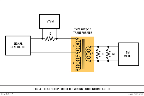
ACHIEVING MAXIMUM SENSITIVITY FOR CONDUCTED EMI CURRENT MEASUREMENTS
The basic circuit in Fig. 2 provides the most pickup and transfer of energy over the frequency range 30 Hz to 150 kHz. Curve #1 of Fig. 3 shows the correction factors required to convert narrowband signals to dB above one µA. Since the sign of the factor is negative for most of the range, the sensitivity is considerably better than that of conventional current probes. The sensitivity achieved by this technique is better than .05 µA at frequencies above 5 kHz when using an EMI meter capable of measuring 1.0 µV into 50 Ω.

FLATTENING THE RESPONSE
At a sacrifice of sensitivity, the upper portion of the frequency versus correction factor curve can be flattened to provide a constant correction factor from about 1 kHz up to 150 kHz. This is depicted in curve #2 of Fig. 3, where a -20 dB correction is suitable over this part of the frequency range. The flattening is obtained by loading the primary with a suitable value or resistance. The resistance value used in this example is 10 Ω. The flattening still allows the measurement of a 0.1 µA signal when using an EMI meter with 1.0 µV sensitivity. An advantage of this response curve is the sloping correction at frequencies below 1 kHz which acts like a high pass filter to remove some of the power line harmonics from wideband measurements. If you are only interested in frequencies above 150 Hz, a 2 Ω resistor is all that is needed. See curve #3.

STILL MORE FLATTENING
The value of the shunt resistor can be reduced even further, resulting in even more loss of sensitivity. This is illustrated in curve #4 of Fig. 3 where a 0.5 Ω shunt resistor is connected across the transformer primary winding used as an output winding to the EMI meter. The overall flatness is achieved at the sacrifice of considerable sensitivity, but the sensitivity is well under the requirements of existing specifications and the correction network utilizes no active elements.

LIMITATIONS OF THE METHOD
When measuring EMI current on DC lines, there are no problems, but on AC lines there are limitations. The AC voltage drop across the winding (S) due to power current flowing to the test sample is the principal problem. This voltage induces twice as much voltage in the output winding (P) at the power frequency. Since we prefer to limit the power dissipation in the 50 Ω input to the EMI meter so that it will not exceed 0.5 W, the induced voltage must be kept below a safe limit. For 400 Hz lines, the power frequency current must not exceed 16 A to avoid too much 400 Hz power dissipation in the input to the EMI meter. Also, the resistance (R) used across the output winding (P) must be at least a 50 W rating on 400 Hz lines. This resistor should be noninductive to avoid errors due to inductive reactance.

DETERMINING THE NARROWBAND CORRECTION FACTOR
The test setup of Fig. 4 describes the simple method of determining either the transfer impedance or the correction curve, whichever is desired. Actually, there is no need to plot the answer as transfer impedance, since the desired end product is the correction factor to be applied to the meter reading to obtain decibels above 1 µA. The correction must be obtained for each configuration. In other words, if you want to use the method for maximum sensitivity, the calibration is performed with just a 50 Ω load on the primary winding simulating the EMI meter. If the flattening networks will be used, then they must be connected to the primary winding during the calibration and must be further loaded with 50 Ω to simulate the EMI meter input. At each test frequency, the output of the audio signal generator is adjusted for a level which delivers the same current to the secondary (S) of the transformer. This is accomplished by setting constant voltage across the 10 Ω resistor. A convenient level is 0.1 V across 10 Ω which is 10,000 µA (80 dB/µA).

Adjust the gain of the EMI meter to assure a 1 µV meter reading for a 1 µV RF input from a standard signal generator. Then connect the 50 Ω input circuit of the EMI meter to the primary of the Solar Type 6220-1B. If the calibration is for maximum sensitivity, no additional loading is necessary. If the calibration is for the flattened versions discussed above, the appropriate resistance must be connected across the primary of the transformer.

At the frequency of the test, set the output of the signal source to obtain 1.0 V across the 10 Ω resistor. Carefully tune the EMI meter to the test frequency and note the meter reading on the dB scale. The difference between the meter reading in dB and 80 dB represents the correction necessary to convert the meter reading to dB above 1 µA for narrowband measurements. In most cases, the correction will have a negative sign. For example, at 100 Hz the EMI meter may read 88 dB above 1 µV. Since the reference is 80 dB above one µA, the correction is -8 dB to be added algebraically to the meter reading to obtain the correct reading in dB above 1 µA.

If the 10 dB pad has been used, this loss must be accounted for in deriving the correction. If the pad will be used in the actual test setups, its loss becomes part of the correction factor. In this case, the meter reading obtained in the foregoing example would be 78 dB above 1 µV and the correction factor would be +2 dB for narrowband measurements.

Repeating this procedure at a number of test frequencies will produce enough data to plot a smooth curve for use when actual tests are being conducted.

DERIVING THE BROADBAND CORRECTION FACTOR
When making broadband measurements as required by MIL-STD-461A in terms of "dB above one µA per MHz," use the average of the narrowband factors over the range 30 Hz to 14 kHz and add a bandwidth correction factor of 37 dB.

In the case of Method CE01 of MIL-STD-461A, use the 20 kHz wideband mode of the EMI meter, determine the average of the narrowband factors over the range 30 Hz to 20 kHz and use this figure as the bandwidth correction factor.

SUMMARY
Some of the material given in this Application Note is terse and given without much explanation. If your are confused by this simplification, just call us. Incidentally, the Signal Corps liked this method so well that they included it in Notice #3 to MIL-STD-462 date 9 Feb. 71.

For background on the development of Solar Electronics transformers, click "History" near the top of this page.